

Vector Database Memory Sizing and Cost Math: How Much RAM Do 1 Million Vectors Need?
Memory math for one million float32, HNSW, SQ8, and PQ vectors; pgvector, Qdrant, and Milvus architectures; production RAM, latency, and cost planning.
· TankDev Mühendislik
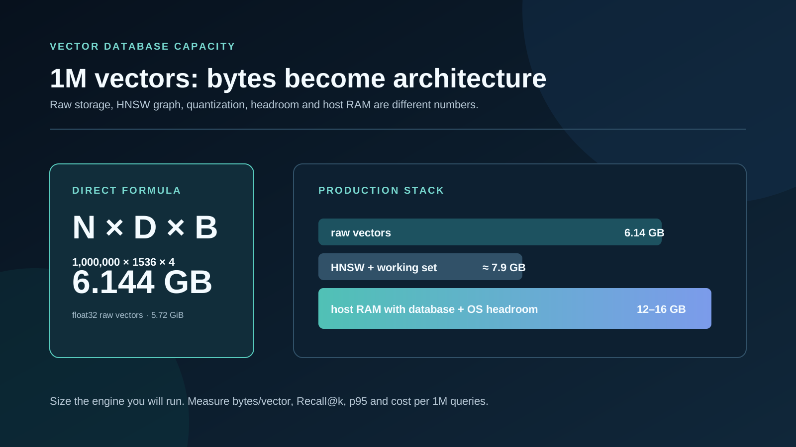
The first vector database memory formula is: raw vector bytes = N × D × B. Use B = 4 bytes for float32, B = 2 for float16, and B = 1 for int8/SQ8. N is the vector count and D is the number of dimensions. Divide by 10^9 for decimal GB or by 2^30 for binary GiB. One million 1536-dimensional float32 vectors therefore require 1,000,000 × 1536 × 4 = 6,144,000,000 bytes, or 6.144 GB / 5.72 GiB of raw vector storage.
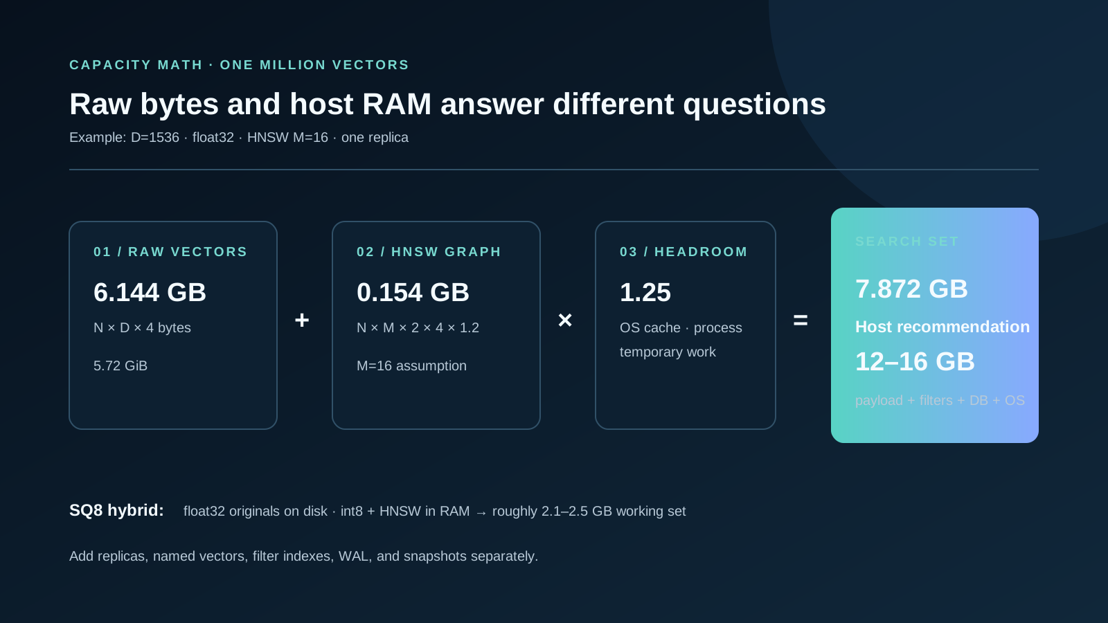
Short answer for one million OpenAI `text-embedding-3-small` vectors: At the default 1536 dimensions and float32 storage, the raw vectors occupy 6.14 GB. With an M=16 HNSW graph and 25% working headroom, the vector-search resident set is approximately 7.9 GB. After PostgreSQL or database processes, metadata, filter indexes, query concurrency, and the operating system, plan at least a 12 GB host, with 16 GB RAM as the safer production tier. If SQ8 stays in RAM while original vectors remain on disk, the search layer can fall to roughly 2.1–2.5 GB, subject to measured recall and p95 latency.
1. Use the correct unit: GB and GiB are not interchangeable
raw_bytes = N × D × bytes_per_dimension
decimal_GB = raw_bytes / 1,000,000,000
binary_GiB = raw_bytes / 1,073,741,824

float32: 4 byte/dimension
float16: 2 byte/dimension
int8 / SQ8: 1 byte/dimension
binary: 1 bit/dimension = 0.125 byte/dimension
Cloud pricing and product pages often use GB, while operating-system tools often display GiB. The same byte count is 6.144 GB or 5.72 GiB, a difference of about 7%. The JSON response size of an embedding API is not the storage size either: textual digits and protocol framing affect transfer, while the database's physical datatype determines storage.
OpenAI's official embeddings guide gives default lengths of 1536 for text-embedding-3-small and 3072 for text-embedding-3-large, and supports shorter outputs through the dimensions parameter. A model name alone therefore does not prove capacity; measure the D value the application actually requests and stores.
2. Size the HNSW graph separately from the vectors
HNSW connects points through a multilayer nearest-neighbour graph. Graph memory scales mainly with vector count, connectivity M, identifier width, and engine layout; raw vector memory scales with N × D. The HNSW paper discusses an implementation-dependent graph cost of roughly 60–450 bytes per object, excluding vector data. There is no universal rule that HNSW is always 20–50% of raw vector size: the percentage looks larger at low dimensions and smaller at 3072 dimensions.
A capacity plan needs an engine-specific approximation. Qdrant's capacity planning guide uses N × M × 2 × 4 bytes × 1.2 for its HNSW graph. The factors represent bidirectional links, four-byte point identifiers, and layering/management allowance. At one million points, this estimates 153.6 MB for M=16 and 307.2 MB for M=32. Another engine can use different pointers, alignment, segments, and copies.
hnsw_graph_bytes ≈ N × M × 2 × 4 × 1.2

N = 1,000,000, M = 16 → 153,600,000 byte = 0.154 GB
N = 1,000,000, M = 32 → 307,200,000 byte = 0.307 GB

resident_search_set ≈ (vector_bytes + graph_bytes + resident_payload_indexes) × headroom3. Comparison table for one million vectors
| Embedding example | D | Raw float32 | HNSW M=16 + 25% | SQ8 + HNSW + 25% | Practical host tier |
|---|---|---|---|---|---|
| All-MiniLM-L6-v2 | 384 | 1.54 GB / 1.43 GiB | ~2.1 GB | ~0.7 GB | 4–8 GB RAM |
| BGE-base class | 768 | 3.07 GB / 2.86 GiB | ~4.0 GB | ~1.2 GB | 8 GB RAM |
| OpenAI text-embedding-3-small (default) | 1536 | 6.14 GB / 5.72 GiB | ~7.9 GB | ~2.1 GB | 12–16 GB RAM |
| OpenAI text-embedding-3-large (default) | 3072 | 12.29 GB / 11.44 GiB | ~15.6 GB | ~4.0 GB | 24–32 GB RAM |
This table is a reproducible starting estimate rather than a purchasing guarantee. M=32, payload indexes, multiple named vectors, tombstones, segment buildup, or an engine that keeps physical vector representations in both the table and index increase the result. Reducing 1536 dimensions to 768 halves raw vector bytes, but retrieval quality still depends on the corpus and query distribution.
4. Worked example: a 1536-dimensional RAG collection
N = 1,000,000
D = 1,536
M = 16

raw_float32 = N × D × 4                 = 6.144 GB
hnsw_graph = N × M × 2 × 4 × 1.2       = 0.154 GB
search_working_set = (6.144 + 0.154) × 1.25 = 7.872 GB

SQ8, originals on disk:
quantized = N × D × 1                   = 1.536 GB
SQ8_working_set = (1.536 + 0.154) × 1.25 = 2.112 GB
The host calculation does not stop there. One million points with an average 1 KB payload add 1 GB of raw payload; not all of it must stay resident, but hot filter indexes might. PostgreSQL sessions can consume work_mem, Qdrant optimizers can create new segments, and Milvus query nodes need temporary room for loading and compaction. Placing a 7.9 GB working set into exactly 8 GB of physical RAM is continuous memory pressure, not capacity planning.
5. Quantization: 75% smaller is real; a fixed quality loss is not
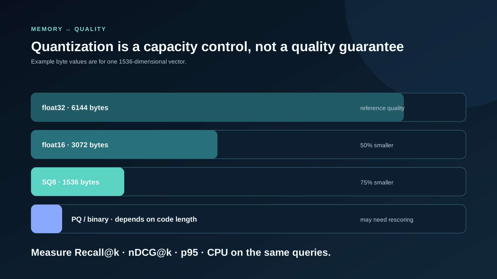
Scalar quantization commonly represents each float32 component with one int8 byte, shrinking the vector copy by about 75%. The system may still keep originals for rescoring, so RAM can fall while disk holds original + quantized copy. Qdrant's quantization documentation describes a hybrid layout with originals on disk and the quantized copy pinned in RAM.
- SQ8 / int8:
Dbytes per vector. SIMD-friendly and usually the first compression profile to test. - float16 / half precision:
2 × Dbytes per vector. Roughly 50% smaller; pgvector can index up to 4000 dimensions withhalfvec. - Binary quantization:
D/8bytes per vector. Very high compression, often used for candidate generation followed by full-precision reranking. - Product quantization:
ceil(subquantizers × bits / 8)bytes per vector plus codebooks. It requires training, tuning, and quality validation.
A claim such as ‘recall falls only 1–2%’ is not portable. Embedding distribution, distance metric, quantile, code length, ef_search/nprobe, filters, and rescoring depth change the outcome. Measure Recall@k, nDCG@k, or task-labelled retrieval. The Faiss index table makes the storage model explicit: HNSW Flat is roughly 4D + links, SQ8 is D, and PQ uses the configured code length per vector.
6. pgvector memory: shared_buffers is not the only cache
pgvector operates inside PostgreSQL's page and index machinery. Every HNSW byte does not have to be pinned inside shared_buffers; PostgreSQL's buffers and the operating-system page cache both participate. The PostgreSQL resource documentation recommends 25% of RAM as a starting point for shared_buffers on a dedicated server and explains that PostgreSQL also relies on the OS cache. effective_cache_size is a planner assumption, not reserved memory.
If hot HNSW pages exceed the combined cache budget, random page faults and storage reads increase. A jump from 5 ms to 400 ms is possible but not universal; NVMe latency, cache hit rate, ef_search, filters, and concurrency determine it. The official pgvector documentation states that HNSW uses more memory than IVFFlat, builds much faster when the graph fits inside maintenance_work_mem, and defaults to M=16, ef_construction=64.
pgvector also has a critical dimensional limit: the vector type supports up to 2000 dimensions for HNSW/IVFFlat, while halfvec supports up to 4000. A default 3072-dimensional text-embedding-3-large result therefore cannot be indexed directly as vector(3072) with HNSW. Request 2000 or fewer dimensions from OpenAI, or build a half-precision halfvec(3072) index, then remeasure retrieval quality on the same evaluation set.
-- Measure the heap and HNSW index independently
SELECT
  pg_size_pretty(pg_relation_size('document_chunks')) AS heap,
  pg_size_pretty(pg_relation_size('document_chunks_embedding_hnsw')) AS hnsw,
  pg_size_pretty(pg_total_relation_size('document_chunks')) AS total;

BEGIN;
SET LOCAL hnsw.ef_search = 100;
EXPLAIN (ANALYZE, BUFFERS)
SELECT id FROM document_chunks
ORDER BY embedding <=> $1
LIMIT 20;
COMMIT;
7. Qdrant and Milvus make placement a design choice
A dedicated vector database differentiates itself not only through ANN algorithms but through placement controls for vectors, HNSW, quantized copies, payloads, and payload indexes. Qdrant's current memory tiers classify structures as pinned, cached, or cold. Cached and cold structures use mmap; the principal difference is whether they are warmed at startup. A cold HNSW graph requires caution because graph traversal performs small random reads. Keeping a quantized copy resident and reading originals only for top-candidate rescoring is often more balanced.
Milvus likewise exposes separate mmap controls in its official configuration for vector fields and vector indexes. These features do not guarantee ‘the same performance with 10× less RAM’. Once the working set exceeds memory, page faults, disk queues, and tail latency can grow. The defensible claim is that dedicated engines offer finer resident-versus-disk placement; the achieved ratio depends on the SSD, query distribution, and quality target.
| Architecture | Memory behaviour | Strength | Risk to measure |
|---|---|---|---|
| PostgreSQL + pgvector | Heap and index pages share PostgreSQL + OS caches | Relational filtering, transactions, one operational surface | Cache contention, high-dimension limits, ANN and write workload overlap |
| Qdrant | Separate tiers for vectors, HNSW, quantized copy, and payload | Hybrid RAM/NVMe placement and ANN operations | Random I/O for cold HNSW; segment/optimizer headroom |
| Milvus | Query-node loading plus vector/index mmap | Distributed scale and a separate query layer | Operational complexity, compaction, per-node loading |
| Faiss / embedded | The chosen index generally lives in the application process | Few services, custom pipelines, batch search | Application owns persistence, metadata, replication, and online updates |
8. Does IVFFlat use less memory than HNSW?
IVFFlat normally has lower index overhead because it does not store graph links. It groups vectors into lists around coarse centroids and scans nprobe lists per query. If it stores full vectors, the raw 4D cost remains. Faiss summarizes IVFFlat as approximately 4D + 8 bytes/vector and HNSW Flat as 4D + graph links. pgvector IVFFlat needs representative data and a suitable lists value; when the distribution changes materially, recall must be remeasured and the index may need rebuilding.
HNSW usually offers a stronger speed–recall trade-off for interactive search and grows online without a training step, in exchange for graph memory, slower builds, and costlier inserts. IVFFlat can suit large, batch-oriented collections with a smaller index overhead. Compare Recall@10, p50/p95/p99, build time, insert throughput, and reindex cost under the same filters.
9. What actually happens when the index does not fit in RAM?
The database does not necessarily stop. Engines using mmap or page cache fetch required pages from disk and evict older pages. HNSW traversal touches scattered neighbours, so every cache miss can add storage latency. When the working set is materially larger than RAM and queries are broadly distributed, major page faults, queue depth, and p99 latency rise together. If swap is active, database heap pages may also be swapped, making the failure mode worse.
- Do not rely on cache hit ratio alone; monitor major page faults, read IOPS, queue depth, and disk latency.
- p50 can remain healthy while p99 collapses; capacity decisions need tail latency.
- Filtered ANN can shrink candidates or reduce recall after filtering; reproduce tenant and category distributions.
- Report cold start, warm cache, and steady state separately.
- Exercise temporary RAM and disk peaks during rebuild, compaction, snapshot, and backup.
10. Replication and shard math
base_vectors = logical_vectors × replication_factor
node_vectors ≈ base_vectors / shard_count × rebalance_headroom

RAM_cluster = resident_bytes_per_vector × base_vectors
RAM_node = RAM_cluster / active_nodes + process_overhead + query_workspace
Disk_cluster = persistent_bytes × replication_factor + WAL + snapshots + temporary_segments
A replication factor of two roughly doubles cluster-wide vector and index copies; two nodes do not automatically halve per-node data. Shards distribute data, while replicas provide resilience. Remaining nodes must absorb query and rebalance load after a failure. Managed-service cost must include replicas, minimum node count, snapshots, network egress, and reindexing hours—not only nominal data size.
11. Turn bytes into monthly cost
monthly_compute = hourly_node_price × 730 × node_count
monthly_storage = provisioned_GB × storage_price_per_GB_month × replicas
monthly_backup = snapshot_GB × retention_copies × backup_price
monthly_total = compute + storage + backup + network + operations

cost_per_1M_queries = monthly_total / monthly_queries × 1,000,000
Forcing the workload onto the smallest RAM instance is not always cheapest. Cold vectors can require a higher IOPS tier, more nodes, or longer query time. PQ saves RAM and disk but can consume more CPU and engineering time. pgvector removes a separate service yet may require a larger PostgreSQL host because transactional traffic and ANN queries share CPU and cache.
| Cost component | Growth variable | Reduction option | Trade-off |
|---|---|---|---|
| Resident RAM | N, D, replicas, HNSW M, filter indexes | Lower D, SQ8/PQ, cold originals | Recall or disk reads |
| NVMe / disk | Original + quantized copy, WAL, snapshots | Retention and segment policy | Recovery window |
| CPU | ef_search, rescoring, concurrency | Smaller candidate set | Recall may fall |
| Operations | Cluster, compaction, backup, upgrade | Consolidate with pgvector or use managed service | Less isolation or control |
| Re-embedding | Chunk count and model/dimension changes | Versioned gradual backfill | Longer migration and dual indexes |
12. Do not make a capacity decision without measurement
The formula gives a physical lower bound; a benchmark reveals the working set. Start with at least hundreds of thousands of representative vectors and approach target scale when possible. Preserve dimensions, norms, languages, chunk lengths, tenant distribution, and metadata filters. Produce exact-search ground truth for a smaller evaluation set and compare ANN output against it.
1. Build ground truth from the same corpus and 500–2,000 real queries.
2. Use identical k, filters, and distance metric for every candidate.
3. Sweep M / ef_construction / ef_search or lists / nprobe.
4. Record Recall@10, nDCG@10, p50, p95, p99, and QPS.
5. Measure warm and cold starts separately.
6. Record RSS, page faults, IOPS, CPU, and index bytes/point.
7. Add concurrent inserts plus rebuild/compaction peaks.
8. Select the lowest total-cost profile that passes the SLO.
Bytes/vector is the strongest capacity comparison unit. Calculate index_size / live_vector_count, then remeasure after tombstones and segment merges. Publish resident_RSS / live_vector_count, p95, Recall@k, and cost_per_1M_queries on the same row. That turns a marketing multiplier into a reproducible engineering decision.
13. Copyable Python sizing calculator
from dataclasses import dataclass

@dataclass
class VectorSizing:
    n: int
    d: int
    bytes_per_dim: float = 4
    m: int = 16
    replicas: int = 1
    headroom: float = 1.25

    def estimate(self):
        base = self.n * self.replicas
        vectors = base * self.d * self.bytes_per_dim
        hnsw = base * self.m * 2 * 4 * 1.2
        resident = (vectors + hnsw) * self.headroom
        return {
            'vector_GB': vectors / 1e9,
            'hnsw_GB': hnsw / 1e9,
            'resident_GB': resident / 1e9,
            'resident_GiB': resident / 2**30,
        }

print(VectorSizing(n=1_000_000, d=1536).estimate())14. Production decision checklist
- Write the actual N, D, datatype, named-vector count, and replication factor.
- Report raw bytes separately in GB and GiB.
- Add graph, payload indexes, process/query workspace, and 25–30% headroom as separate lines.
- Choose SQ8 or PQ from your ground-truth queries, not a claimed universal recall loss.
- For pgvector, combine heap/index size, EXPLAIN ANALYZE BUFFERS, and cache-pressure metrics.
- For Qdrant/Milvus, document placement of vectors, graph, quantized copy, and payloads.
- Test whether the SLO survives node loss and rebalancing.
- Put cost per 1M queries beside recall and p95 in the final decision table.
TankDev's RAG versus fine-tuning guide explains which problem the retrieval layer should solve; our API and system integration guide shows how that layer joins a reliable production flow. Explore our applied AI engineering service, or share your corpus size, embedding model, target recall, and latency so the estimate can become a measured capacity plan.
Frequently asked questions
01How much RAM do one million OpenAI vectors need?
One million default 1536-dimensional text-embedding-3-small vectors occupy 6.144 GB as float32. With an M=16 HNSW graph and 25% working headroom, the search resident set is about 7.9 GB. Allowing for database processes, metadata, filter indexes, and the OS, plan at least 12 GB and preferably a 16 GB production host. SQ8 in RAM with originals on disk can reduce the search layer to roughly 2.1–2.5 GB.
02How much storage do one million 3072-dimensional vectors use?
The float32 raw size is 12.288 GB or 11.44 GiB. With M=16 HNSW and 25% working headroom, the search set is about 15.6 GB. Payloads, processes, and index-building headroom make a 24–32 GB RAM host a more realistic production starting point.
03What happens when a vector index does not fit in RAM?
The engine may continue through mmap or page cache, but scattered HNSW access increases cache misses, major page faults, IOPS, and especially p99 latency. A 10× or 100× slowdown is possible but not fixed; it depends on NVMe latency, ef_search, filters, concurrency, and query locality.
04Does HNSW always add 20–50% over raw vector memory?
No. Graph cost scales mostly with N and M, while raw vector cost scales with N and D. The same graph is a larger percentage at 384 dimensions than at 3072. Engine-specific layers, pointers, alignment, and metadata also matter. Use bytes-per-vector math and measured index size instead of a universal percentage.
05Does scalar quantization lose only 1–2% recall?
There is no universal bound. Loss depends on the embedding distribution, metric, quantile, candidate depth, and rescoring. It can be negligible on one corpus and material on another. Measure Recall@k or nDCG@k on the same labelled queries before selecting it.
06Does IVFFlat use less memory than HNSW?
IVFFlat usually has lower index overhead because it stores no graph links, although full-vector storage still costs 4D bytes. HNSW often provides a stronger interactive speed–recall trade-off at the cost of graph memory and slower builds. IVFFlat requires training and recall validation as the distribution changes.
07Must a pgvector HNSW index fit entirely in shared_buffers?
No. PostgreSQL uses both shared_buffers and the operating-system page cache, while effective_cache_size is only a planner estimate. Hot pages exceeding the combined cache budget still cause disk reads and tail-latency growth. Measure heap/index size separately and test real queries with EXPLAIN ANALYZE BUFFERS.
08Do Qdrant or Milvus guarantee 10× less RAM in on-disk mode?
No. They provide more flexible placement of vectors, graph, and payload. The saving depends on quantization, cache locality, SSD, and query distribution. Lower RAM can require more disk I/O, CPU rescoring, or higher p99 latency.
09Does halving embedding dimensions halve total RAM?
It roughly halves raw vectors and SQ8 copies, but an HNSW graph with the same N and M remains similar. Total process memory therefore may fall by less than 50%. Retrieval quality must also be remeasured at the shorter dimension.
10Which metrics should compare vector database cost?
Use the same corpus and query set to compare Recall@k or nDCG@k, p50/p95/p99, QPS, bytes/vector, resident RSS, build time, insert throughput, and cost per 1M queries. Add replicas, snapshots, reindexing, and operational effort to total cost.